The most important math you should learn!

“The journey of solving a problem is often more rewarding than the solution itself.” Terence Tao

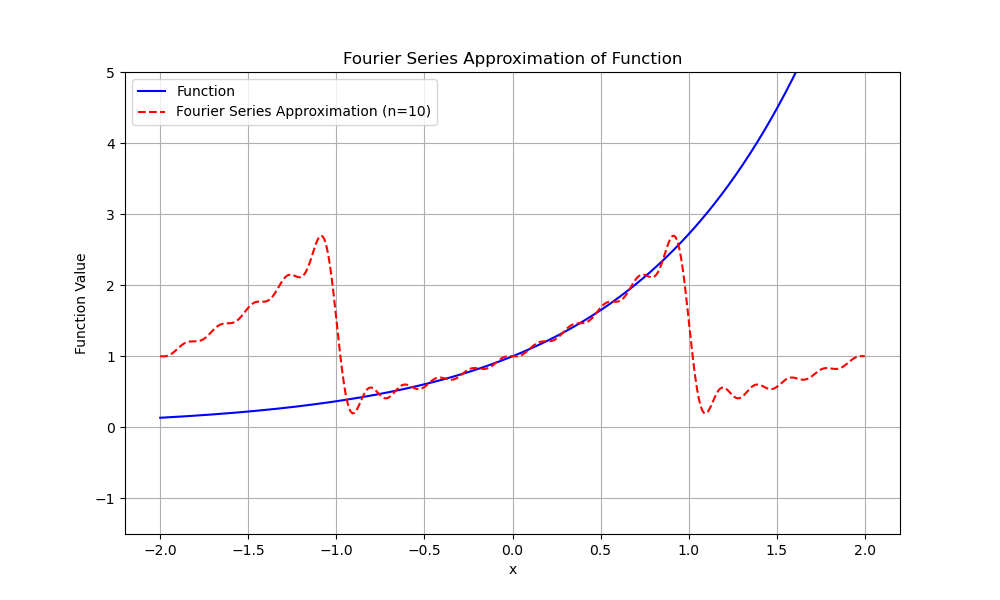
A Fourier series(see figure 1) is an expansion of a periodic function into a sum of trigonometric functions(sines and cosines). Quite hard to understand, right? If I were you, my brain would explode just thinking about all those technical terms linked together (proven through research!). But my goal as a student is to shorten the gap of understanding efficiently, using less mental power. And I claim that understanding

‘orthogonality’ will make you grasp the rest of the Fourier series(fourier techniques). But how, you ask? Let’s start with a story!

The Tale of the Orchestra and the Conductor

Once upon a time, in a land where music was the essence of life, there was a grand orchestra. This orchestra was unique because each musician played a pure, distinct tone—a sine wave of a specific frequency.

The orchestra was led by a wise and experienced conductor who had the extraordinary ability to create any piece of music by combining the tones played by the musicians. However, the conductor faced a significant challenge: the music created by combining all these tones often turned into a confusing cacophony, making it hard to identify and adjust individual contributions.

One day, the conductor discovered an ancient musical manuscript that described the secret of orthogonality. According to the manuscript, orthogonality was like a magical property that would allow the conductor to separate and manage each tone independently, even when they were all playing together.

Individual Contributions: The manuscript revealed that each musician’s tone was orthogonal to the others. This meant that if one musician’s tone was represented by a sine wave of a certain frequency, it had no overlap or interference with the tones of other musicians. Mathematically, the inner product (a way to measure overlap) of different sine waves was zero.

Magical Filters: Armed with this knowledge, the conductor could now use special mathematical filters to extract each musician’s contribution from the combined music. These filters were like magic spells that could isolate one tone from the blend, allowing the conductor to hear and analyze each musician’s part as if they were playing alone.

Reconstruction of Music: With the ability to separate and manage each tone, the conductor could now reconstruct any piece of music by adjusting the volume (amplitude) and timing (phase) of each musician’s tone independently. This made it possible to create harmonious and complex compositions without the parts interfering with one another.

Balance and Harmony: The conductor used the orthogonality principle to balance the orchestra perfectly. By understanding that each tone was independent, the conductor could adjust each musician’s contribution to achieve the desired overall sound, ensuring harmony and clarity in every performance.

The musicians in the orchestra also benefited from this understanding. They realized that by playing their tones correctly and in tune with the orthogonality principle, they contributed to the beauty of the music without clashing with their peers.

Moral of the Story: In the realm of Fourier series, the sine and cosine functions (the musicians) are orthogonal. This orthogonality means that each sine and cosine function at different frequencies does not interfere with one another when we analyze a complex signal. The “conductor” (the mathematician or engineer) can use this property to:

Decompose a complex signal into its fundamental sine and cosine components. Analyze each component separately to understand its contribution. Reconstruct the original signal by combining these components appropriately.

Orthogonality in Fourier series ensures that we can manage and manipulate each frequency component independently, leading to clear and accurate analysis and synthesis of signals. This principle is crucial for many applications in engineering, physics, and beyond.

We engineers often face difficult real-life problems, especially in mathematics, which we don’t seem to excel at naturally. The actual work is different from the theory because teachers usually provide problems that are well-defined, but in practice, things can be more complex. You need to apply your math skills in every case and in certain situations. In any case, the Fourier series technique is very useful to us If one has honed its judgment.

Before we delve into the technical part of the Fourier series. One must always know the history and its development to how it became to what it is today. For the lack of a better term, this is just how I learn and understand things.

Historical Development: The Journey of Fourier Series

Things always set in motion in the pursuit of discovery! Now, Imagine it’s the early 19th century, and you’re a French mathematician named Joseph Fourier. You’re fascinated by the problem of heat conduction and how heat spreads through different materials. To tackle this, you propose a radical idea: representing a function describing the temperature distribution as a sum of simpler, periodic functions—sines and cosines.

Despite skepticism from your peers, you published your work in 1822, titled “Théorie analytique de la chaleur” (The Analytical Theory of Heat). You show that complex, periodic heat distributions can be broken down into a series of simpler waves. This idea, the Fourier series, begins to slowly gain acceptance.

The Foundations Strengthened A few decades later, other mathematicians like Peter Gustav Lejeune Dirichlet came along and provided rigorous proofs to support your work. Dirichlet formulates the conditions under which these series converge, giving the mathematical community the confidence that your method works under specific circumstances.

Applications in Physics and Engineering Fast forward to the late 19th and early 20th centuries. Mathematicians and physicists, including Henri Poincaré, begin to apply Fourier series to various fields. Poincaré uses them to solve complex problems in celestial mechanics, studying the stability of orbits of planets and stars. Fourier series help break down the periodic motion of celestial bodies into manageable components, aiding in the understanding of gravitational interactions. Meanwhile, in Germany, David Hilbert introduces the concept of Hilbert spaces, providing a more general and abstract framework for understanding functions and series, including Fourier series. This development allows mathematicians to handle infinite-dimensional spaces with the same confidence as finite-dimensional ones.

Transforming Technology: The Fast Fourier Transform (FFT) The story takes a revolutionary turn in 1965. Two American mathematicians, James Cooley and John Tukey, develop the Fast Fourier Transform (FFT), an algorithm that dramatically speeds up the computation of Fourier series. This innovation makes it feasible to use Fourier analysis in real-time applications. With FFT, Fourier series become a cornerstone of digital signal processing. Engineers can now efficiently analyze and filter signals in various technologies—radios, televisions, and telephones. FFT transforms the telecommunications industry, enabling the compression and transmission of data over long distances without losing quality.

The Digital Age: From Medical Imaging to Audio Engineering As we enter the digital age, the applications of Fourier series continue to expand. Medical professionals use them in MRI scans to create detailed images of the inside of the human body. By analyzing the frequency components of the signals received from the scanner, doctors can diagnose diseases with high precision. In the music industry, Fourier series and the FFT enable audio engineers to manipulate sound recordings. They can isolate and remove noise, enhance certain frequencies, and create digital effects, revolutionizing music production and sound design.

The development of Fourier series is rooted in the contributions of several key figures: D’Alembert: Introduced the 1-dimensional wave equation, describing the vibrations of a string using trigonometric functions.

Bernoulli: Proposed that the motion of a vibrating string could be described as a superposition of sinusoidal functions.

Fourier: Introduced the idea that any periodic function could be represented by an infinite series of sine and cosine functions, although initially lacking rigorous mathematical foundation.

Cauchy: Addressed convergence issues of Fourier series, providing a more rigorous mathematical framework and defining conditions under which the series converges.

Dirichlet: Provided the first rigorous proof of Fourier’s theorem, establishing conditions (Dirichlet conditions) for the convergence of Fourier series.

Riemann: Expanded Fourier’s work to study the integrability and convergence of series.

Hilbert: Developed the concept of Hilbert space, providing a general framework for understanding functions and series, emphasizing orthogonality, inner product, and completeness.

Mathematical principles: Periodic Signals: Fourier series are particularly useful for analyzing periodic signals. Continuous Time and Discrete Frequency Transformation: Fourier series provide a way to transform a continuous-time signal into a discrete set of frequency components.

Decomposition of Functions: Breaking down complex functions into simpler sine and cosine components.

Orthogonality: Basis functions (sines and cosines) are orthogonal, meaning they do not overlap, which simplifies the computation of coefficients.

Inner Product: Projecting functions onto basis functions to find the coefficients of the series.

Convergence and Completeness: Conditions under which the series converges to the function, and the idea that every function in a space can be represented as an infinite series of basis functions.

Weighting Function: Determines the contribution of each sinusoidal component to the overall periodic function.

Discrete Spectrum: Defined at multiples of the fundamental frequency for periodic signals.

Now that we know how the fourier series works under the hood and how it is developed through the years, let’s look for its development and practical applications.

Applications:

1. Heat Equation Application: Solving the heat distribution in a given domain over time. Orthogonality and Linearity: The heat equation is a linear partial differential equation (PDE). When solving it using separation of variables, the resulting solutions are often in the form of orthogonal functions (e.g., sine and cosine functions in a bounded domain). These orthogonal functions allow us to decompose the initial heat distribution into simpler components, solve for each component independently, and then sum the solutions to get the overall heat distribution.

2. Harmonic Analysis Application: Analyzing vibrations and waveforms in mechanical and electrical systems. Orthogonality and Linearity: Harmonic analysis involves breaking down complex waveforms into their fundamental sinusoidal components (harmonics). These components are orthogonal sine and cosine functions, which simplifies the analysis and synthesis of the waveform. This approach is linear because the principle of superposition applies, allowing each harmonic to be treated independently.

3. Signal Processing Application: Filtering, compressing, and analyzing signals (e.g., audio, video, communications). Orthogonality and Linearity: In signal processing, the Fourier transform(development of fourier series) decomposes signals into orthogonal sinusoidal components. This orthogonality allows efficient filtering and compression, as each frequency component can be manipulated independently. Linearity ensures that the superposition principle holds, enabling the combination of processed components to reconstruct the original or modified signal accurately.

4. Image Compression (e.g., JPEG, MPEG) Application: Reducing the file size of images and videos. Orthogonality and Linearity: Image compression algorithms like JPEG use the Discrete Cosine Transform (DCT) to convert image data into frequency components. These components are orthogonal, allowing for efficient separation and quantization of the image data. Linearity ensures that the superposition principle applies, enabling the accurate reconstruction of the image from its compressed components.

5. Modal Analysis in Structural Engineering Application: Determining the natural vibration modes of structures. Orthogonality and Linearity: In modal analysis, the natural vibration modes (eigenmodes) of a structure are calculated. These modes are orthogonal to each other, meaning each mode represents an independent way the structure can vibrate. The linearity of the equations of motion ensures that the superposition of these modes accurately describes the overall vibration behavior of the structure.

6. Chirped Pulse Amplification

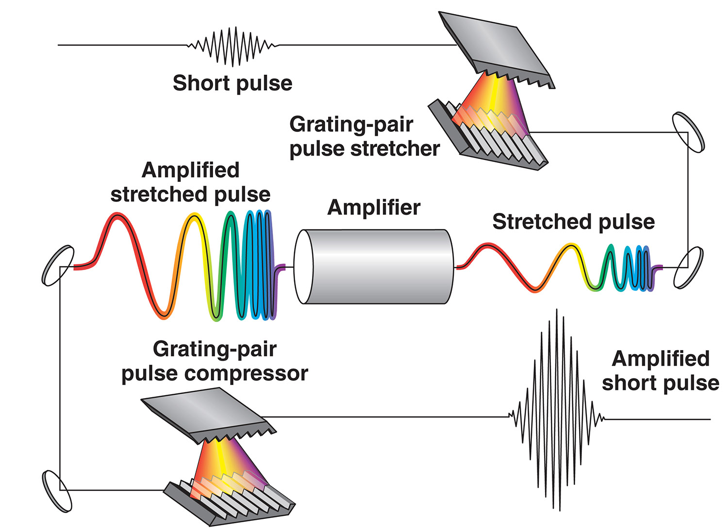
Application: Enabled the creation of extremely powerful laser systems Orthogonality and Linearity: involves stretching an ultra-short laser pulse in time, amplifying it, and then compressing it back to its original duration. This process allows the amplification of pulses to extremely high peak powers without damaging the amplifying medium.

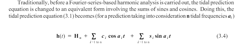
1. Tidal analysis and prediction Application: periodic nature of tides, allowing their representation as a sum of sinusoidal components. machines like wave energy converter is useful to this Orthogonality and Linearity: accurate decomposition of tidal data into constituent frequencies, while the linearity property enables the combination of different tidal constituents to model complex tidal patterns effectively

Each of these examples leverages the orthogonality and linearity of functions to simplify complex problems, allowing for efficient analysis, manipulation, and reconstruction of systems and signals.

It’s good to know its application but how do we do things in real life? 1 real life engineering story about its application.

The Challenge of Noise Reduction in Audio Signals

Imagine it’s the mid-20th century, and you’re working as an audio engineer at a music recording studio. You and your team face a recurring problem: the recordings are often distorted by unwanted noise. This noise could come from various sources—mechanical vibrations, electrical interference, or even environmental sounds. The challenge is to clean up these recordings without losing the quality of the music.

Initial Attempts: Analog Filters

Initially, your team tries using analog filters to reduce the noise. While these filters can help, they are not very precise. They often remove parts of the actual music along with the noise, leading to a loss of quality. You need a more sophisticated method to separate the noise from the music.

Enter Fourier Series

One day, a mathematician visits your studio and suggests using a mathematical technique called Fourier series. The idea is to break down the complex audio signal into simpler components—sine and cosine waves. Each of these waves represents a different frequency component of the original signal.

The mathematician explains that any periodic signal, like your music recording, can be expressed as a sum of these sine and cosine waves. By analyzing the frequency components, you can identify and isolate the unwanted noise.

Applying Fourier Series: The Solution

You decide to give it a try. Here’s how you proceed:

Digitizing the Signal: First, you convert the analog audio recording into a digital signal. This involves sampling the continuous audio signal at regular intervals to create a sequence of discrete data points.

Fourier Transform: Next, you apply the Fourier transform(next level of fourier series) to the digital signal. This mathematical operation transforms the time-domain signal (the original audio recording) into the frequency domain. In the frequency domain, you can see the amplitudes of the different frequency components that make up the audio signal.

Identifying Noise:

By examining the frequency spectrum, you notice certain frequency components that are abnormally high and don’t correspond to the musical notes. These are the noise frequencies.

Filtering Out Noise:

You then create a digital filter that removes these unwanted frequency components. This process involves setting the amplitudes of the noise frequencies to zero or significantly reducing them.

Inverse Fourier Transform: Finally, you apply the inverse Fourier transform to convert the filtered signal back into the time domain. The result is a cleaner audio recording with significantly reduced noise.

Summary

Fourier series connect abstract mathematics with real-world applications, showcasing their significant impact and utility. This highlights the power of mathematical insight to drive innovation and shape our world.

It is almost always important to note that:

1. [Seek] Idealized problems ->[Find] General solutions -> [Create] Realistic models

2. Where there’s curvature in space, there’s change in time

3. Constraints that the temperature function must satisfy if it’s going to accurately describe heat flow.

4. Boundary conditions

5. Initial condition - because you don’t get to choose how it looks at t = 0

6. Gain control of this ocean turning all of the right knobs and dial, so as to select from it the particular solution fitting a given initial conditions

7. Differential equations offer us a really nice context where you can see how that plays out

TLDR: now you know the following(I hope so :D)

-Define what a Fourier series is and understand why its formula is the way it is.

-Explain the concept of orthogonality in the context of sine and cosine functions

-Identify real-world applications of Fourier series in various fields such as engineering, physics, and signal processing.